Introduction
We’re in the home stretch, folks! Welcome to my last blog update for the 2024 presidential election, which less than two weeks away. This week, we discussed “shocks,” a broad category of external factors and events that aren’t the result of campaigns or systematic fundamental forces. Such shocks can range from pandemics to natural disasters and local college football victories, all with potential implications for voter behavior — depending on who you ask.
In this blog, I briefly discuss the role of shocks in presidential elections and continue to update my national and state-level models in preparation for my final prediction!
Assessing Shocks
The effects of shocks on elections are perhaps best understood through the logic of retrospection, where voters look to the past to assess incumbent performance. To Christopher Achen and Larry Bartels, voters’ supposed reactions to shocks paint a bleak picture for democracy: voters are swayed by irrelevant factors — such as shark attacks — and fail to accurately evaluate the current government and incumbent. Andrew Healy and Neil Malhotra likewise finds that voters punish incumbents for random events (droughs, floods, economic shocks, etc) and fail to differentiate between government-caused outcomes and uncontrollable external factors. Following this perspective, shocks and their impact on voting behavior undermine the democratic ideal of elections as accountability mechanisms.
However, there’s also evidence to prove that shocks don’t truly have a predictive effect on election outcomes. Marco Mendoza and Semra Sevi find that COVID-19 exposure didn’t consistently affect voting — pre-existing partisan identities had a much stronger role.
Let’s quickly revisit the polling visualization with potential “game-changers” from Blog 3. Here is the updated plot with national polling averages to the date of this blog’s writing (October 24, 2024).
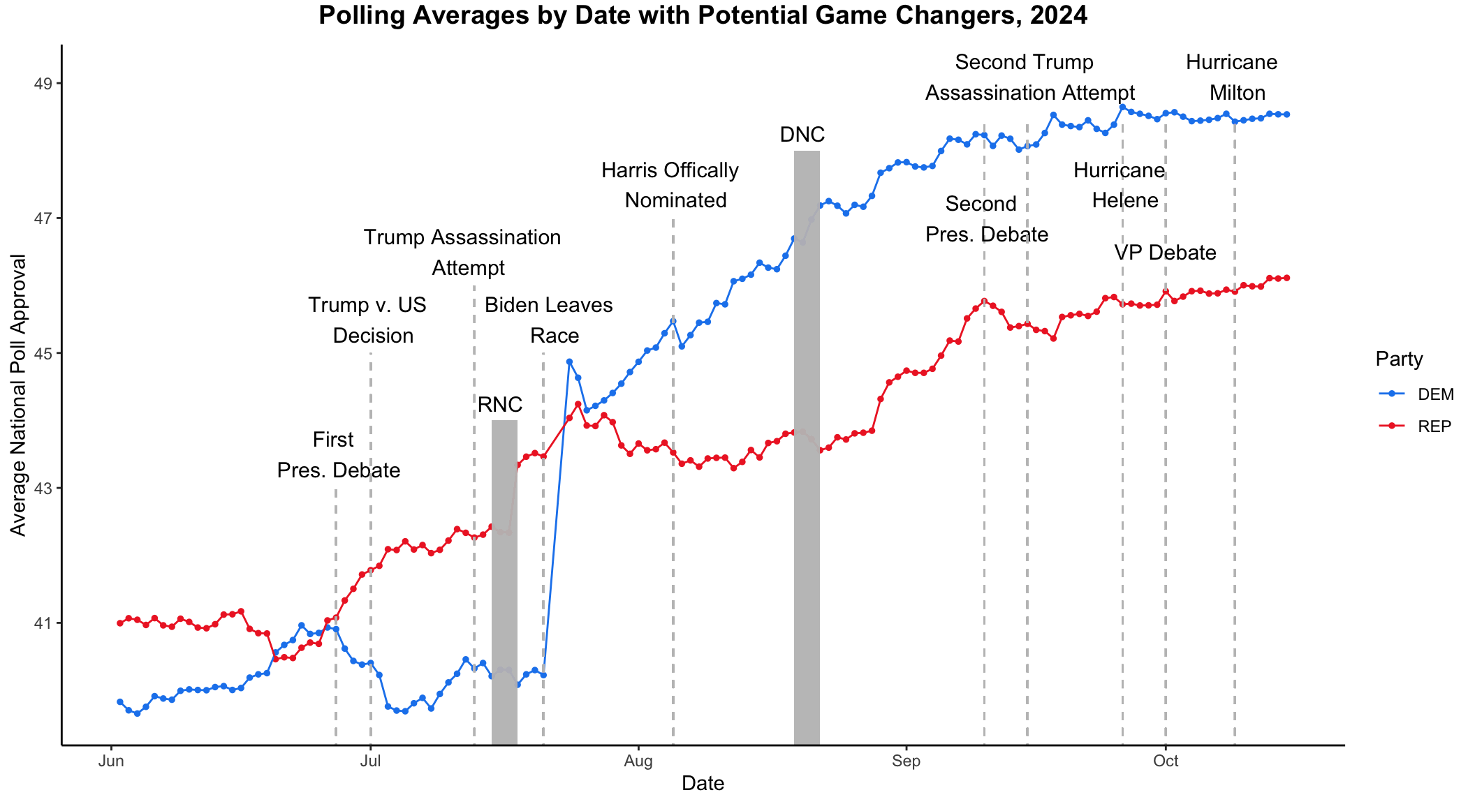
Again, it is difficult to establish a causal relationship between potential “game-changers” and trends in public opinion. That being said, polling doesn’t seem to change much following these events. Perhaps it’s because America has become so politically calcified that such “shocks” don’t affect us: we’ll still be voting for our party’s candidate at the end of the day. It’s interesting to think about what would happen if we put the craziness of the 2024 election cycle in the context of another presidential election year — would these potential “game-changers” have more of a notable effect?
To conclude this discussion on shocks, I briefly look at the potential effect of hurricanes on electoral outcomes. For this graph, I plot a regression between the number of hurricanes in a presidential election year (occurring before November) and the two-party popular vote share for the incumbent party’s candidate.
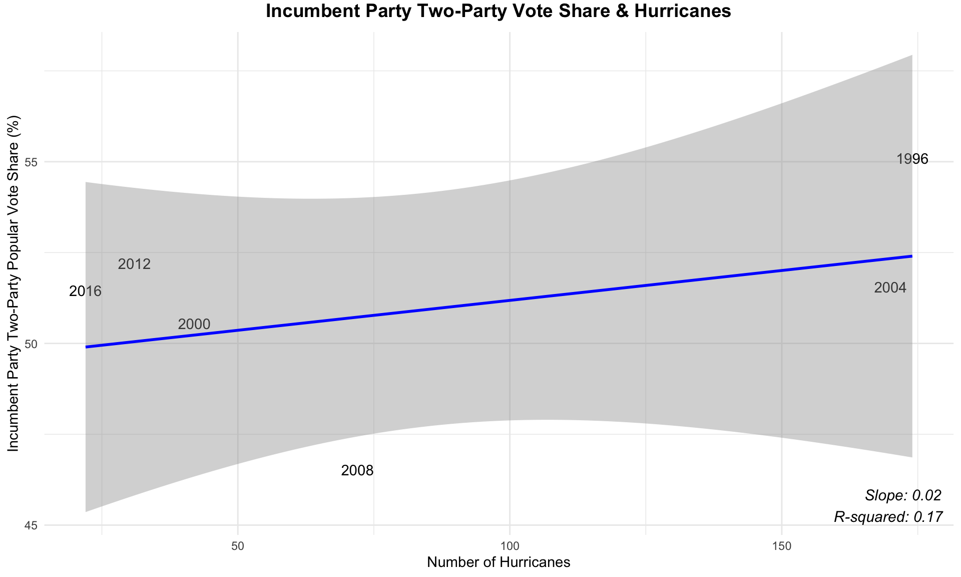
For this regression, the slope of the line of best fit is barely greater than 0 and the R-squared value of 0.17 is low. This seems to indicate that there isn’t a strong relationship between the number of hurricanes in a presidential election year and the two-party popular vote for the incumbent party’s candidate. Specifically, the low R-squared value indicates that only a small portion of vote share variation is explained by the number of hurricanes, implying that other factors likely play a much larger role in influencing election outcomes.
So, do shocks matter for presidential election outcomes? The answer is obviously complicated, but these two simple analyses seem to signal that they do not.
National Two-Party Popular Vote Model
For this week’s national model, I test a different combination of the factors that I’ve been using previous weeks: quarterly GDP growth for Q2 of the election year, national October polling averages (weighted by weeks left before the election), national two-party percentage of voters, and an incumbent variable (1 if the incumbent party candidate was also the incumbent president, 0 if not). The regression table is below!
| National Popular Vote Share for Incumbent Party Candidate | ||||
|---|---|---|---|---|
| Predictors | Estimates | std. Error | CI | p |
| (Intercept) | 21.77 | 5.19 | 9.81 – 33.74 | 0.003 |
| GDP growth quarterly | 0.50 | 0.14 | 0.18 – 0.82 | 0.007 |
| oct poll | 0.47 | 0.08 | 0.29 – 0.64 | <0.001 |
| two party percent | 0.12 | 0.06 | -0.02 – 0.26 | 0.093 |
| incumbent | 1.13 | 1.08 | -1.36 – 3.61 | 0.327 |
| Observations | 13 | |||
| R2 / R2 adjusted | 0.920 / 0.880 | |||
The model has an R-squared value of 0.92 and R-squared adjusted value of 0.88, which suggests that it is a strong predictor for the incumbent party candidate’s national two-party popular vote share. Here, Q2 GDP growth and October national polling averages are statistically significant predictors, while two-party percent and incumbent status aren’t statistically significant. Once again, we only have polling data up to the date of this blog’s writing (October 24, 2024). I now use this model to predict Vice President Harris’ (the incumbent party candidate) share of the national two-party popular vote.
| Prediction | Lower Bound | Upper Bound |
|---|---|---|
| 52 | 47.49 | 56.52 |
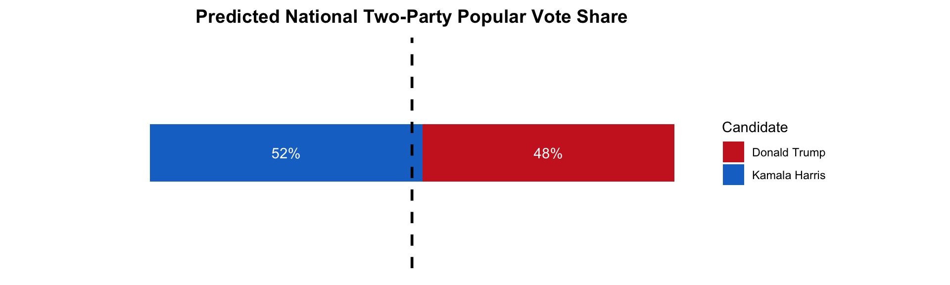
Similar to last week, this model predicts that Harris will win 52% of the national two-party popular vote. The prediction intervals are also smaller here than the previous two weeks!
Next, let’s assess the out-of-sample fit for this model. I performed 1,000 runs of a cross-validation, randomly selecting half of the election years in my data set to test the model each run. Here, the mean of the absolute value of the out-of-sample residuals was approximately 3.63. Considering that the national two-party vote share spans nearly 20 points, this suggests a positive indication of the model’s performance. This histogram displays the distribution of out-of-sample errors for this week’s national model.
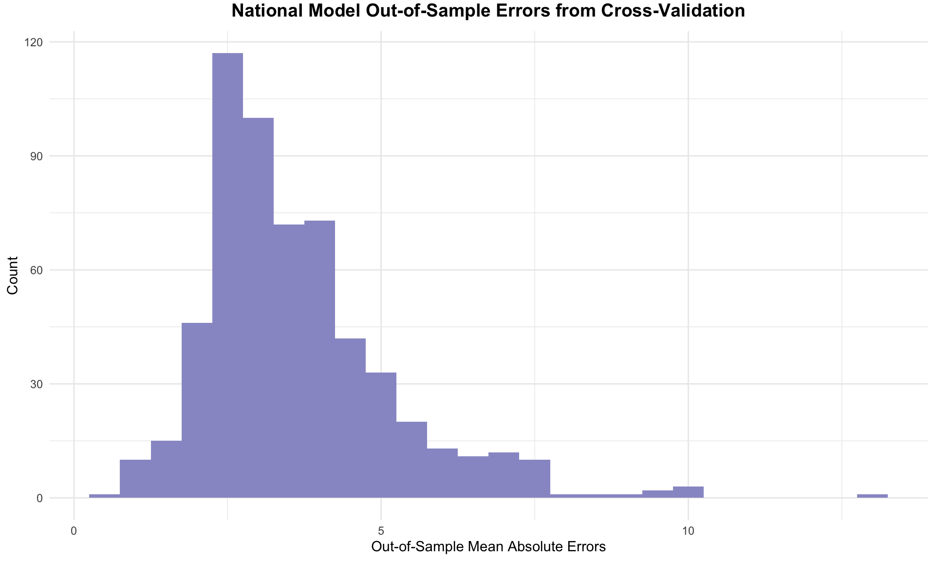 The errors appear slightly right-skewed, indicating the model occasionally underestimates the incumbent party's performance by a wider margin than it overestimates.
Here is a summary visualization for this week’s prediction of the national two-party popular vote! The dashed black line indicates 50% of the national popular vote.
State Two-Party Popular Vote Model & Electoral College Prediction
Moving onto my state-level model, I utilize September state polling averages, October state polling averages, and an indicator for the incumbent party (1 if an incumbent party candidate, 0 if not) as coefficients. Not bounded by the campaign events data of last week, I train the model on presidential elections from 2000 to 2020. The regression table for the Democratic candidate’s state-level popular vote share is below.
| Democrat's State-Level Popular Vote Share | ||||
|---|---|---|---|---|
| Predictors | Estimates | std. Error | CI | p |
| (Intercept) | -2.33 | 1.11 | -4.52 – -0.14 | 0.037 |
| sept poll | -0.31 | 0.14 | -0.57 – -0.04 | 0.024 |
| oct poll | 1.43 | 0.13 | 1.17 – 1.69 | <0.001 |
| incumbent party | 2.57 | 0.39 | 1.81 – 3.33 | <0.001 |
| Observations | 290 | |||
| R2 / R2 adjusted | 0.894 / 0.893 | |||
Higher than last week, the R-squared values of 0.89 indicate the model’s strong fit. All the coefficients here are statistically significant. October polling is a strong positive predictor of the Democratic state-level popular vote share with the incumbent variable also a significant positive coefficient. On the other hand, September polling is a negative, slightly smaller coefficient, indicating that higher September polling averages slightly reduce the predicted Democratic vote share — which seems counter-intuitive. This may indicate some noise in earlier polls or possible overemphasis on early polling that might shift by Election Day.
This is the state model’s prediction for our 13 states of interest.
| State | Prediction | Lower Bound | Upper Bound | Winner |
|---|---|---|---|---|
| Arizona | 50.26 | 43.89 | 56.62 | Harris |
| Florida | 48.89 | 42.52 | 55.26 | Trump |
| Georgia | 50.72 | 44.35 | 57.09 | Harris |
| Michigan | 51.56 | 45.19 | 57.93 | Harris |
| Minnesota | 53.75 | 47.38 | 60.13 | Harris |
| Nevada | 51.59 | 45.22 | 57.96 | Harris |
| New Hampshire | 55.08 | 48.70 | 61.45 | Harris |
| New Mexico | 54.03 | 47.66 | 60.41 | Harris |
| North Carolina | 50.95 | 44.58 | 57.31 | Harris |
| Pennsylvania | 51.69 | 45.32 | 58.06 | Harris |
| Texas | 47.41 | 41.04 | 53.78 | Trump |
| Virginia | 54.11 | 47.74 | 60.48 | Harris |
| Wisconsin | 51.83 | 45.46 | 58.21 | Harris |
Like last week, this model predicts that Harris will win 11 out of the 13 states, with Trump winning Florida and Texas again. The electoral margin continues to decrease from week to week (e.g. Pennsylvania 51.69% this week vs 51.79% in Blog 7 and 52.86% in Blog 6) with smaller prediction intervals as well. Obviously, these races are still extremely close and most of the prediction intervals include 50%.
To visualize this, I calculate the predicted win margin for Harris in the 13 state races with their confidence intervals, sorted by greatest to smallest predicted margin. Since I’m calculating the predicted win margin for the Democratic candidate, a negative win margin favors the Republican candidate. The black dot is the predicted win margin, with the blue dot (favoring Democrats) representing the upper bound and the red dot (favoring Republicans) representing the lower bound of the win margin.

New Hampshire, Virginia, and New Mexico have the highest predicted win margins for Harris. Close states include Arizona, Georgia, and North Carolina. Pennsylvania is higher on this chart than I would’ve expected — it currently sits in the middle of the pack with very similar margins to the other swing states of Michigan, Nevada, Wisconsin, and Minnesota.
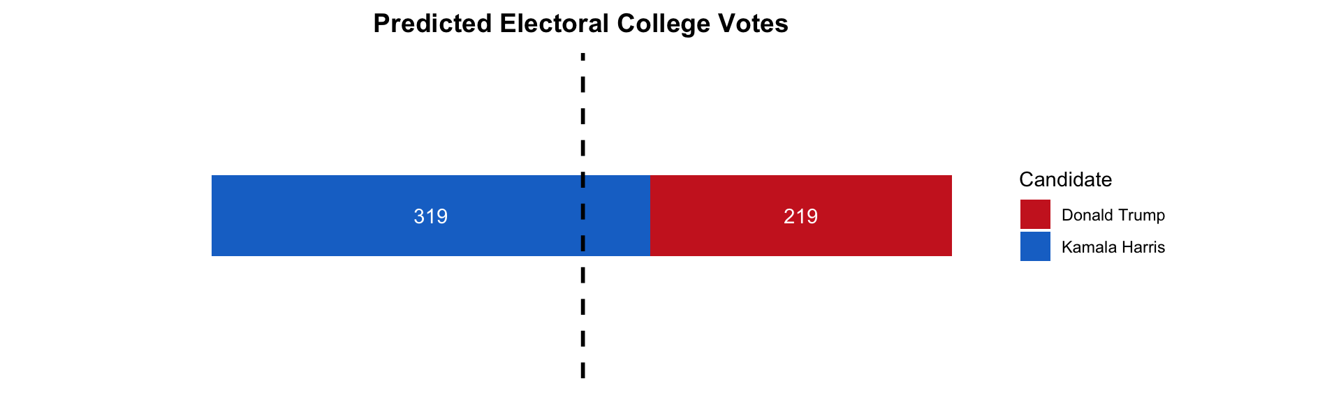
Incorporating in the other states, here is this week’s Electoral College map!
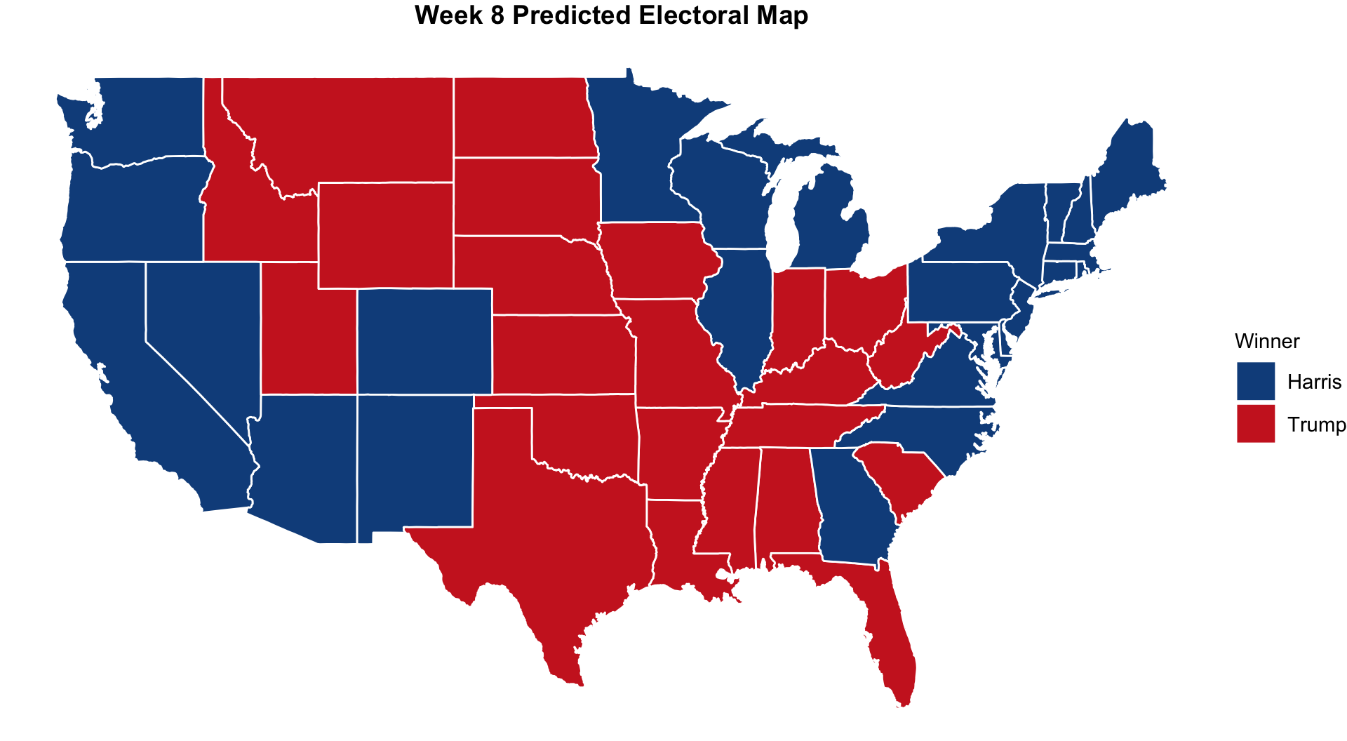
Similar to the state prediction, I create another visualization to summarize the Electoral College prediction for this week. The dashed black line indicates 270 electoral votes, which is the number of votes required to win the Electoral College.
Conclusion
Once again, I predict that Harris will win both the national two-party popular vote and the Electoral College. We’re less than 14 days away from the election, so I’m excited (and a little scared) to see how our predictions will shake out. Looking forward to putting together my final election prediction next week!