Introduction
From canvassing to phone banks, the second main aspect of presidential campaigns is the “ground game.” The on-the-ground efforts of political organizing require a completely different set of infrastructure than the “air war” discussed in last week’s blog: campaigns must work to identify and selectively target individual voters, while coordinating thousands of volunteers and field offices across the country. Former President Barack Obama’s 2008 campaign against the late Senator John McCain is widely considered to have revolutionized the modern conceptualization of the ground game — we know that this side of the campaigning effects voting behavior to a certain extent.
In this penultimate blog update, I first examine historical trends in “ground game” mobilization — specifically campaign events and field offices — across the 2012-2024 presidential elections. I pay particular attention to the states and geographical regions targeted by these campaigning efforts. Then, I transition to updating my models to predict the national two-party popular vote and the Electoral College for the quickly-approaching 2024 election.
Campaign Events
Arguably, the “ground game” of campaigns is most visibility manifested in campaign events, including rallies, speeches, and town halls. To start, I examine the number of campaign events over time for the 2016, 2020, and 2024 (so far) presidential elections — the visualization is below.
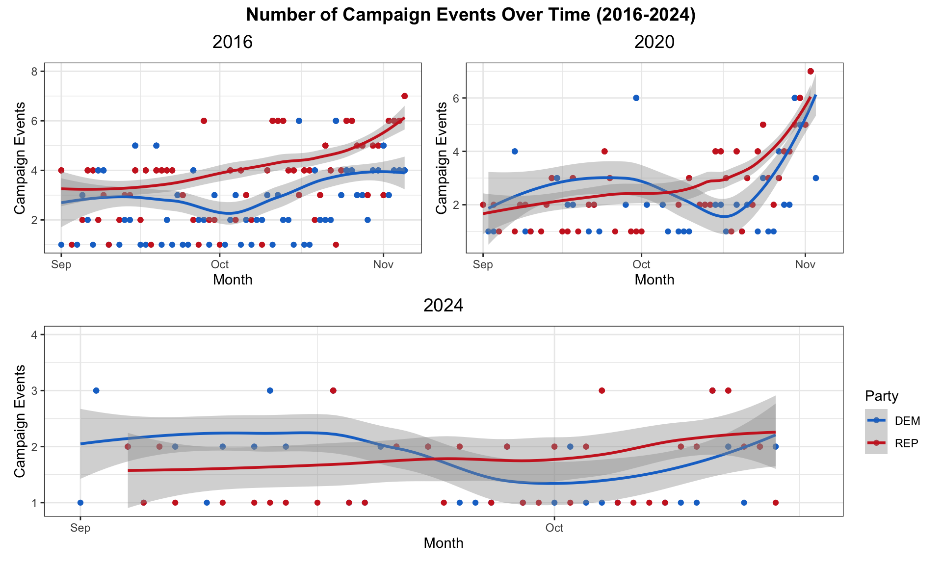
As expected, the number of campaign events for both parties increases over time. While 2016 and 2020 exhibit a sharp increase in campaign events approaching Election Day, the 2024 trend remains relatively flat with fewer events overall, particularly for the Republican candidate.
I also map the location of these campaign events for each of the 3 election cycles. Each circle represents a campaign event, colored blue if hosted by the Democratic candidate and red for the Republican candidate.
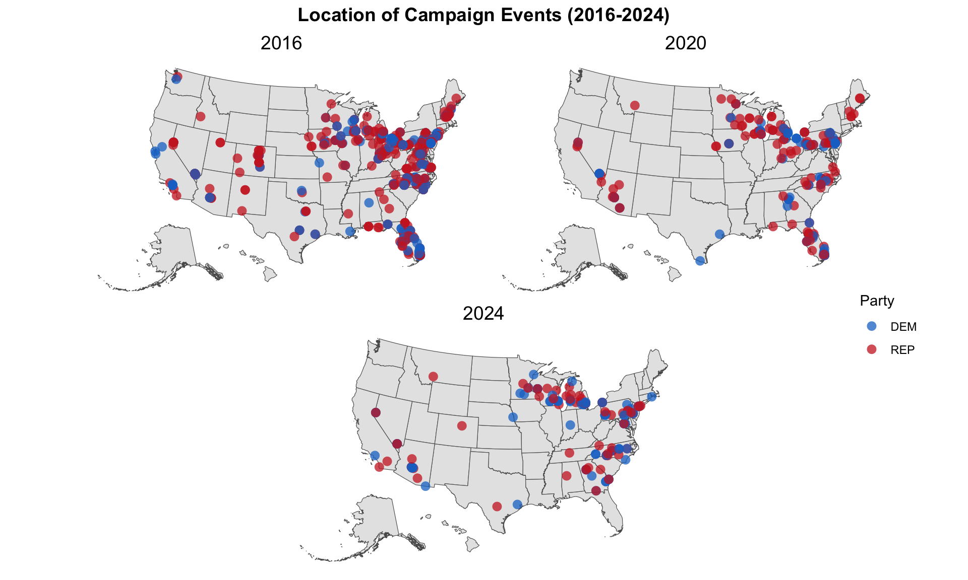
Looking at these maps, there seems to be a lot of geographic overlap in the locations that campaigns choose to host their events. Many campaign events take place in the Great Lakes region (near the “blue wall” states of Michigan and Wisconsin) as well as the Mid-Atlantic and southern states along the East Coast. The density of dots appears to be the highest and most geographically spread in 2016, which indicates a larger number of campaign events held over a greater number of states. In comparison, campaign events in 2024 seem to have concentrated in a handful of states so far, including Wisconsin, Michigan, Pennsylvania, Georgia, and Pennsylvania.
The following table presents the number of campaign events in our 13 states of interest for 2024 over the past 3 presidential elections. The final row of the table displays the total number of events across all these states for each campaign.
| State | Clinton | Trump | Biden | Trump | Harris | Trump |
|---|---|---|---|---|---|---|
| Arizona | 3 | 6 | 3 | 10 | 7 | 5 |
| Florida | 44 | 40 | 14 | 17 | 0 | 0 |
| Georgia | 0 | 3 | 4 | 3 | 9 | 6 |
| Michigan | 9 | 16 | 10 | 10 | 13 | 10 |
| Minnesota | 1 | 2 | 2 | 6 | 3 | 2 |
| Nevada | 9 | 10 | 5 | 6 | 6 | 3 |
| New Hampshire | 7 | 15 | 0 | 4 | 0 | 0 |
| New Mexico | 0 | 3 | 0 | 0 | 0 | 0 |
| North Carolina | 24 | 32 | 6 | 14 | 10 | 10 |
| Pennsylvania | 25 | 32 | 23 | 20 | 14 | 11 |
| Texas | 4 | 5 | 2 | 0 | 1 | 1 |
| Virginia | 8 | 22 | 0 | 1 | 0 | 1 |
| Wisconsin | 7 | 10 | 6 | 12 | 10 | 8 |
| TOTAL EVENTS | 141 | 196 | 75 | 103 | 73 | 57 |
By simply looking at the total events row, we see that the 2016 presidential election had the highest number of campaign events in these states. Former President Trump beat both Secretary Clinton and President Biden in terms of the volume of campaign events in these states for 2016 and 2020, although Vice President Harris holds a slight advantage in 2024 thus far. On the individual state level, it’s interesting to note that neither candidate has hosted a campaign event in Florida for the 2024 electoral cycle, despite the high number of events in previous elections. Also, at this point in the cycle, the number of campaign events in Georgia has more than doubled from the 2020 election for both parties. Once again, the battleground states of Michigan, North Carolina, and Pennsylvania have attracted significant campaign attention across all 3 elections.
I decided to take a closer look at Pennsylvania, which is one of the most important battleground states in the 2024 contest. This is a county-level map of Pennsylvania, where the fill color of each county indicates the margin by which the Democratic or Republican candidate won that county in 2020 — a more intense blue or red symbolizes a wider margin of victory for the appropriate party. Over this map, I’ve also plotted the location of 2024 campaign events by party so far. Some of these circles are overlapped on top of each other — meaning that the candidates hosted events in the same city — and that is represented by a darker blue/purple colored circle.
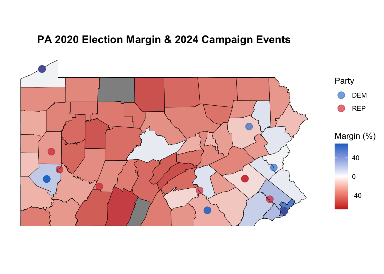
So far, both 2024 candidates have hosted events in Philadelphia and Erie. I think it’s important to examine campaign activity in the lighter colored counties, which indicates a narrower win margin in 2020. For example, the Harris campaign has hosted events in York county and Luzerne county (both won by Trump in 2020) and in Lehigh county and Northampton county (narrowly won by Biden in 2020). The Trump campaign has likewise hosted an event in the counties surrounding Philadelphia, which went for Biden in 2020. To some extent, this map is evidence that campaigns pay attention to previous election results to inform future campaign investments.
Field Offices
Next, I survey past trends in the location and number of campaign field offices. We only have data on field offices for 2012 and 2016, so the geographical spread of field offices for those two election cycles is mapped below.
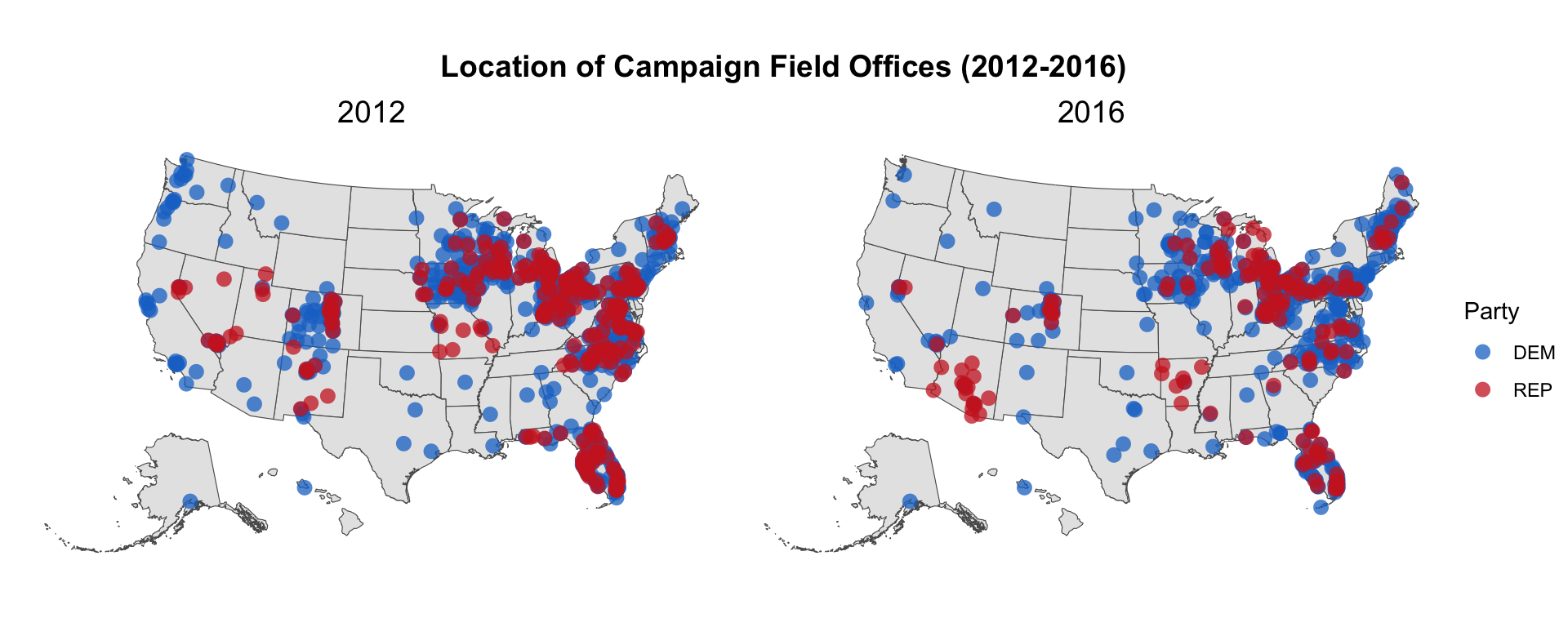
The field offices follow a similar pattern as the campaign events, concentrating along the West/East coasts and the Great Lakes region. At face value, the density of offices seem quite similar across both elections, perhaps with less offices across both parties in 2016 relative to 2012. Notably, we see a clear growth of Republican field offices in Arizona from 2012 to 2016.
The next table displays the number of field offices in the 13 states for the 2012 and 2016 presidential elections. Again, the final row of the table provides the total number of field offices across all these states for each campaign.
| State | Obama | Romney | Clinton | Trump |
|---|---|---|---|---|
| Arizona | 2 | 0 | 2 | 18 |
| Florida | 104 | 48 | 69 | 23 |
| Georgia | 4 | 0 | 1 | 1 |
| Michigan | 28 | 24 | 27 | 22 |
| Minnesota | 12 | 0 | 13 | 0 |
| Nevada | 26 | 12 | 16 | 3 |
| New Hampshire | 22 | 9 | 26 | 6 |
| New Mexico | 13 | 8 | 1 | 0 |
| North Carolina | 54 | 24 | 35 | 8 |
| Pennsylvania | 54 | 25 | 57 | 12 |
| Texas | 4 | 0 | 6 | 0 |
| Virginia | 61 | 29 | 33 | 6 |
| Wisconsin | 69 | 24 | 40 | 13 |
| TOTAL OFFICES | 453 | 203 | 326 | 112 |
Overall, the total number of field offices in these states seems to have dropped from 2012 to 2016. Exceptions include the increase in Republican field offices in Arizona (+18) and Georgia (+1), as well as the increase in Democratic field offices in Minnesota (+1), New Hampshire (+4), Pennsylvania (+3), and Texas (+2) — not significantly large increases.
National Two-Party Popular Vote Model
I now transition to updating my national two-party popular vote prediction. For this week’s national model, I exclude Q2 RDI quarterly growth and the national two-party percentage of voters included in Blog 6. Instead, I add the national October polling averages (weighted by weeks left before the election) as another coefficient. The regression table for this week’s national popular vote share model is below.
| National Popular Vote Share for Incumbent Party Candidate | ||||
|---|---|---|---|---|
| Predictors | Estimates | std. Error | CI | p |
| (Intercept) | 30.87 | 3.75 | 22.22 – 39.52 | <0.001 |
| GDP growth quarterly | 0.45 | 0.17 | 0.07 – 0.83 | 0.025 |
| sept poll | -0.21 | 0.28 | -0.87 – 0.45 | 0.484 |
| oct poll | 0.61 | 0.26 | 0.01 – 1.22 | 0.048 |
| incumbent | 1.00 | 1.27 | -1.94 – 3.93 | 0.456 |
| Observations | 13 | |||
| R2 / R2 adjusted | 0.891 / 0.836 | |||
The model has an R-squared value of 0.89 and R-squared adjusted value of 0.84, which suggests that it is a strong predictor for the incumbent party candidate’s national two-party popular vote share. Of note here is that Q2 GDP growth and October national polling averages are statistically significant predictors of the incumbent party candidate’s vote share, while September polling averages and incumbent status are not statistically significant. Again, we only have data on polling averages up to the date of this blog’s writing (October 17, 2024). I use this model to predict Harris’ share of the national two-party popular vote.
| Prediction | Lower Bound | Upper Bound |
|---|---|---|
| 51.88 | 46.6 | 57.16 |
In a slight decrease from previous weeks, this model predicts that Harris will win the national two-party popular vote by approximately 51.9%. Perhaps this national model comes closer to conveying the tightly contested nature of this year’s presidential election — for context, Biden defeated Trump 51.3% to 46.9% in 2020. The prediction intervals are also smaller here than the previous two weeks, which is a good sign.
| Candidate | Two-Party Popular Vote Share (%) |
|---|---|
| Kamala Harris | 51.88 |
| Donald Trump | 48.12 |
State Two-Party Popular Vote Model & Electoral College Prediction
Next up is updating the state model. This week, I add campaign events data — the total number of events in a given state — to the state model from Blog 6. Since we only have campaign events data from 2016 on, this state-level model is limited to 2016-2020, which is important to keep in mind. The regression table for the Democratic candidate’s state-level popular vote share follows.
| Democrat's State-Level Popular Vote Share | ||||
|---|---|---|---|---|
| Predictors | Estimates | std. Error | CI | p |
| (Intercept) | 2.28 | 2.46 | -2.60 – 7.16 | 0.356 |
| sept poll | -0.49 | 0.36 | -1.20 – 0.22 | 0.172 |
| oct poll | 1.52 | 0.34 | 0.85 – 2.20 | <0.001 |
| campaign events | 0.01 | 0.07 | -0.13 – 0.15 | 0.940 |
| Observations | 96 | |||
| R2 / R2 adjusted | 0.820 / 0.814 | |||
In this model, only October state-level polling averages are a statistically significant predictor of the Democrat’s state-level popular vote share. The R-squared value of 0.82 and adjusted R-squared value of 0.81 indicate that the model has a relatively good fit. Here is this model’s 2024 prediction for our 13 states of interest:
| State | Prediction | Lower Bound | Upper Bound | Winner |
|---|---|---|---|---|
| Arizona | 50.37 | 41.18 | 59.56 | Harris |
| Florida | 49.15 | 39.98 | 58.32 | Trump |
| Georgia | 50.80 | 41.58 | 60.02 | Harris |
| Michigan | 51.61 | 42.32 | 60.89 | Harris |
| Minnesota | 53.56 | 44.37 | 62.76 | Harris |
| Nevada | 51.72 | 42.55 | 60.90 | Harris |
| New Hampshire | 54.75 | 45.53 | 63.97 | Harris |
| New Mexico | 53.79 | 44.57 | 63.00 | Harris |
| North Carolina | 51.05 | 41.83 | 60.28 | Harris |
| Pennsylvania | 51.79 | 42.49 | 61.08 | Harris |
| Texas | 47.74 | 38.56 | 56.91 | Trump |
| Virginia | 53.92 | 44.72 | 63.12 | Harris |
| Wisconsin | 51.76 | 42.51 | 61.02 | Harris |
This week’s state model predicts that Harris will win 11 out of 13 states, while Trump wins Florida and Texas. Harris’ margins of victory are smaller here (e.g. Michigan at 51.61% this week vs 52.93% in Blog 6), and the prediction intervals are slightly larger relative to last week. Personally, I feel a little more at ease that this model predicted Trump to win Florida — given the current state of the polls, I doubt that Harris will be able to flip the state as last week’s state model predicted.
Adding back in the other states, we get the following Electoral College map for this week’s model.
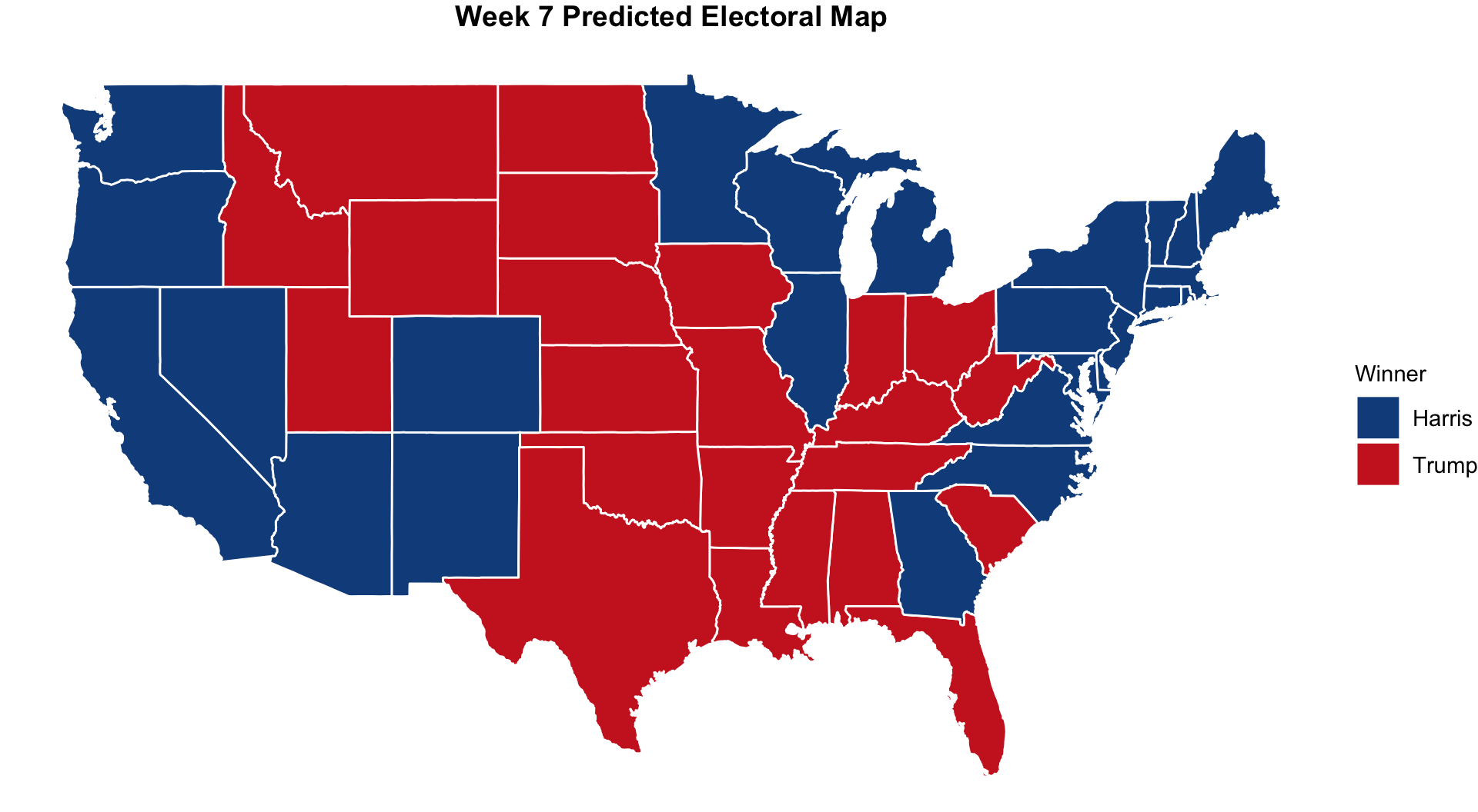
Here is the predicted tally for the Electoral College votes!
| Candidate | Electoral College Votes |
|---|---|
| Kamala Harris | 319 |
| Donald Trump | 219 |
Conclusion
Another week, another predicted presidential victory for Harris. A few thoughts moving into next week: I think that removing Q2 RDI growth in the national model was a good decision (in terms of its statistical insignificance and for the sake of reducing over-fitting), so that coefficient may not return for my final national model. For the state model, incorporating data on campaign events decreased the number of observations and only allowed me to train the model on 2 presidential elections. It could be argued here that narrowing down the state model to Trump-era races is productive, given that today’s political environment is a very different world from that of the early 2000s. However, I’m not sure if I’ll continue to incorporate campaign-related data into my models moving forward — they generally appear to be weaker predictors of vote share and tend to vary greatly from candidate to candidate. Onward!